Principal component analysis (PCA) is routinely employed on a wide range of problems. From the detection of outliers to predictive modeling, PCA has the ability of projecting the observations described by variables into few orthogonal components defined at where the data ‘stretch’ the most, rendering a simplified overview. PCA is particularly powerful in dealing with multicollinearity and variables that outnumber the samples ().

It is an unsupervised method, meaning it will always look into the greatest sources of variation regardless of the data structure. Its counterpart, the partial least squares (PLS), is a supervised method and will perform the same sort of covariance decomposition, albeit building a user-defined number of components (frequently designated as latent variables) that minimize the SSE from predicting a specified outcome with an ordinary least squares (OLS). The PLS is worth an entire post and so I will refrain from casting a second spotlight.

In case PCA is entirely new to you, there is an excellent Primer from Nature Biotechnology that I highly recommend. Notwithstanding the focus on life sciences, it should still be clear to others than biologists.

Mathematical foundation

There are numerous PCA formulations in the literature dating back as long as one century, but all in all PCA is pure linear algebra. One of the most popular methods is the singular value decomposition (SVD). The SVD algorithm breaks down a matrix of size  into three pieces,

where  is the matrix with the eigenvectors of ,  is the diagonal matrix with the singular values and  is the matrix with the eigenvectors of . These matrices are of size ,  and , respectively. The key difference of SVD compared to a matrix diagonalization () is that  and  are distinct orthonormal (orthogonal and unit-vector) matrices.

PCA reduces the dimensions of your data set down to principal components (PCs). The scores from the first PCs result from multiplying the first columns of with the  upper-left submatrix of . The loading factors of the PC are directly given in the  row in . Consequently, multiplying all scores and loadings recovers . You might as well keep in mind:

• PCs are ordered by the decreasing amount of variance explained
• PCs are orthogonal i.e. uncorrelated to each other
• The columns of should be mean-centered, so that the covariance matrix
• SVD-based PCA does not tolerate missing values (but there are solutions we will cover shortly)

For a more elaborate explanation with introductory linear algebra, here is an excellent free SVD tutorial I found online. At any rate, I guarantee you can master PCA without fully understanding the process.

Let’s get started with R

Although there is a plethora of PCA methods available for R, I will only introduce two,

• prcomp, a default function from the R base package
• pcaMethods, a Bioconductor package that I frequently use for my own PCAs

I will start by demonstrating that prcomp is based on the SVD algorithm, using the base svd function.

By default, prcomp will retrieve PCs. Therefore, in our setting we expect having four PCs.The svd function will behave the same way:

Now that we have the PCA and SVD objects, let us compare the respective scores and loadings. We will compare the scores from the PCA with the product of and from the SVD. In R, matrix multiplication is possible with the operator %*%. Next, we will directly compare the loadings from the PCA with from the SVD, and finally show that multiplying scores and loadings recovers . I rounded the results to five decimal digits since the results are not exactly the same! The function t retrieves a transposed matrix.

PCA of the wine data set

Now that we established the association between SVD and PCA, we will perform PCA on real data. I found a wine data set at the UCI Machine Learning Repository that might serve as a good starting example.

According to the documentation, these data consist of 13 physicochemical parameters measured in 178 wine samples from three distinct cultivars grown in Italy. Let’s check patterns in pairs of variables, and then see what a PCA does about that by plotting PC1 against PC2.

Among other things, we observe correlations between variables (e.g. total phenols and flavonoids), and occasionally the two-dimensional separation of the three cultivars (e.g. using alcohol % and the OD ratio).

If its hard enough looking into all pairwise interactions in a set of 13 variables, let alone in sets of hundreds or thousands of variables. In these instances PCA is of great help. Let’s give it a try in this data set:

Three lines of code and we see a clear separation among grape vine cultivars. In addition, the data points are evenly scattered over relatively narrow ranges in both PCs. We could next investigate which parameters contribute the most to this separation and how much variance is explained by each PC, but I will leave it for pcaMethods. We will now repeat the procedure after introducing an outlier in place of the 10th observation.

As expected, the huge variance stemming from the separation of the 10th observation from the core of all other samples is fully absorbed by the first PC. The outlying sample becomes plain evident.

PCA of the wine data set with pcaMethods

We will now turn to pcaMethods, a compact suite of PCA tools. First you will need to install it from the Bioconductor:

There are three mains reasons why I use pcaMethods so extensively:

• Besides SVD, it provides several different methods (bayesian PCA, probabilistic PCA, robust PCA, to name a few)
• Some of these algorithms tolerate and impute missing values
• The object structure and plotting capabilities are user-friendly

All information available about the package can be found here. I will now simply show the joint scores-loadings plots, but still encourage you to explore it further.

I will select the default SVD method to reproduce our previous PCA result, with the same scaling strategy as before (UV, or unit-variance, as executed by scale). The argument scoresLoadings gives you control over printing scores, loadings, or both jointly as right next. The standard graphical parameters (e.g. cex, pch, col) preceded by either letters s or l control the aesthetics in the scores or loadings plots, respectively.

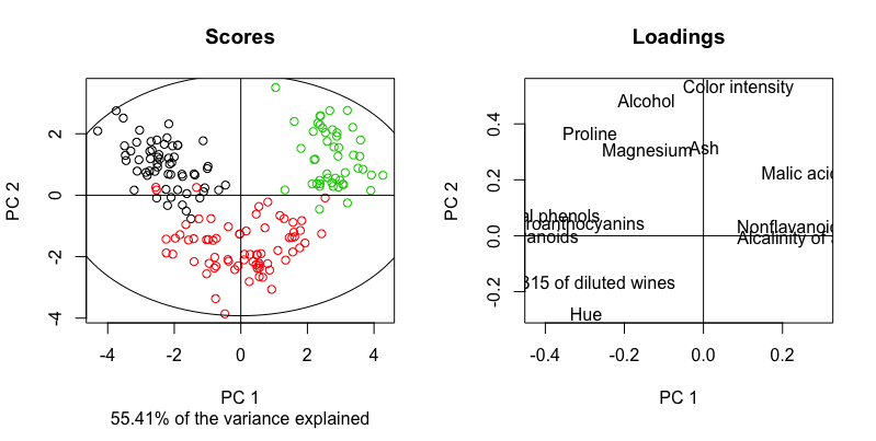
So firstly, we have a faithful reproduction of the previous PCA plot. Then, having the loadings panel on its right side, we can claim that

• Wine from Cv2 (red) has a lighter color intensity, lower alcohol %, a greater OD ratio and hue, compared to the wine from Cv1 and Cv3.
• Wine from Cv3 (green) has a higher content of malic acid and non-flavanoid phenols, and a higher alkalinity of ash compared to the wine from Cv1 (black)

Finally, although the variance jointly explained by the first two PCs is printed by default (55.41%), it might be more informative consulting the variance explained in individual PCs. We can call the structure of winePCAmethods, inspect the slots and print those of interest, since there is a lot of information contained. The variance explained per component is stored in a slot named R2.

Seemingly, PC1 and PC2 explain 36.2% and 19.2% of the variance in the wine data set, respectively. PCAs of data exhibiting strong effects (such as the outlier example given above) will likely result in the sequence of PCs showing an abrupt drop in the variance explained. Screeplots are helpful in that matter, and allow you determining how much variance you can put into a principal component regression (PCR), for example, which is exactly what we will try next.

PCR with the housing data set

Now we will tackle a regression problem using PCR. I will use an old housing data set also deposited in the UCI MLR. Again according to its documentation, these data consist of 14 variables and 504 records from distinct towns somewhere in the US. To perform PCR all we need is conduct PCA and feed the scores of PCs to a OLS. Let’s try predicting the median value of owner-occupied houses in thousands of dollars (MEDV) using the first three PCs from a PCA.

The printed summary shows two important pieces of information. Firstly, the three estimated coefficients (plus the intercept) are considered significant (). Second, the predictability as defined by the  (coefficient of determination, in most cases the same as the squared Pearson correlation coefficient) was 0.63.

Next we will compare this simple model to a OLS model featuring all 14 variables, and finally compare the observed vs. predicted MEDV plots from both models. Note that in the lm syntax, the response is given to the left of the tilde and the set of predictors to the right. Moreover, provided there is an argument for data you can circumvent the need for typing all variable names for a full model (), and simply use . .

Here the full model displays a slight improvement in fit (). The high significance of most coefficient estimates is suggestive of a well-designed experiment. Nevertheless, it is notable that such a reduction of 13 down to three covariates still yields an accurate model.

Just as a side note, you probably noticed both models underestimated the MEDV in towns with MEVD worth 50,000 dollars. My guess is that missing values were set to MEVD = 50.

Concluding,

• The SVD algorithm is founded on fundamental properties of linear algebra including matrix diagonalization. SVD-based PCA takes part of its solution and retains a reduced number of orthogonal covariates that explain as much variance as possible.
• Use PCA when handling high-dimensional data. It is insensitive to correlation among variables and efficient in detecting sample outliers.
• If you plan to use PCA results for subsequent analyses all care should be undertaken in the process. Although typically outperformed by numerous methods, PCR still benefits from interpretability and can be effective in many settings.

All feedback from these tutorials is very welcome, please enter the Contact tab and leave your comments. I do also appreciate suggestions. Enjoy!

 

 

• R