

My last entry introduces principal component analysis (PCA), one of many unsupervised learning tools. I concluded the post with a demonstration of principal component regression (PCR), which essentially is a ordinary least squares (OLS) fit using the first 
- There is virtually no limit for the number of predictors. PCA will perform the decomposition no matter how many variables you handle. Simpler models such as OLS do not cope with more predictors than observations (i.e.
).
- Correlated predictors do not undermine the regression fit. Collinearity is a problem for OLS, by widening the solution space, i.e. destabilizing coefficient estimation. PCA will always produce few uncorrelated PCs from a set of variables, correlated or not.
- The PCs carry the maximum amount of variance possible. In any predictive model, predictors with zero or near-zero variance often constitute a problem and behave as second intercepts. In the process of compression, PCA will find the projections where your data points spread out the most, thus facilitating learning from the subsequent OLS.
However, in many cases it is much wiser performing a decomposition similar to the PCA, yet constructing PCs that best explain the response, be it quantitative (regression) or qualitative (classification). This is the concept of partial least squares (PLS), whose PCs are more often designated latent variables (LVs), although in my understanding the two terms can be used interchangeably.
PLS safeguards advantages 1. and 2. and does not necessarily follow 3. In addition, it follows that if you use the same number of 
Today we will perform PLS-DA on the Arcene data set hosted at the UCI Machine Learning Repository that comprises 100 observations and 10,000 explanatory variables (
Let’s get started with R
For predictive modelling I always use the caret package, which builds up on existing model packages and employs a single syntax. In addition, caret features countless functions that deal with pre-processing, imputation, summaries, plotting and much more we will see firsthand shortly.
For some reason there is an empty column sticking with the data set upon loading, so I have added the colClasses argument to get rid of it. Once you load the data set take a look and note that the levels of most proteins are right-skewed, which can be a problem. However, the authors of this study conducted an exhaustive pre-processing and looking into this would take far too long. The cancer / no-cancer labels (coded as -1 / 1) are stored in a different file, so we can directly append it to the full data set and later use the formula syntax for training the models.
| # Load caret, install if necessary | |
| library(caret) | |
| arcene <- read.table("http://archive.ics.uci.edu/ml/machine-learning-databases/arcene/ARCENE/arcene_train.data", | |
| sep = " ", | |
| colClasses = c(rep("numeric", 10000), "NULL")) | |
| # Add the labels as an additional column | |
| arcene$class <- factor(scan("https://archive.ics.uci.edu/ml/machine-learning-databases/arcene/ARCENE/arcene_train.labels", | |
| sep = "\t")) |
We can finally search missing values (NA’s). If these were present it would require some form of imputation – that is not the case. Calling any(is.na(arcene)) should prompt a FALSE.
So now the big questions are:
- How accurately can we predict whether a patient is sick based of the MS profile of his/her blood serum?
- Which proteins / MS peaks best discriminate sick and healthy patients?
Time to get started with the function train. With respect to pre-processing we will remove zero-variance predictors and center and scale all those remaining, in this exact order using the preProc argument. Considering the size of the sample (n = 100), I will pick a 10x repeated 5-fold cross-validation (CV) – a large number of repetitions compensates for the high variance stemming from a reduced number of folds – rendering a total of 50 estimates of accuracy. Many experts advise in favor of simpler models when performance is undistinguishable, so we will apply the “one SE” rule that selects the least complex model with the average cross-validated accuracy within one standard error (SE) from that in the optimal model. Finally, we must define a range of values for the tuning parameter, the number of LVs. In this particular case we will consider all models with 1-20 LVs.
| # Compile cross-validation settings | |
| set.seed(100) | |
| myfolds <- createMultiFolds(arcene$class, k = 5, times = 10) | |
| control <- trainControl("repeatedcv", index = myfolds, selectionFunction = "oneSE") | |
| # Train PLS model | |
| mod1 <- train(class ~ ., data = arcene, | |
| method = "pls", | |
| metric = "Accuracy", | |
| tuneLength = 20, | |
| trControl = control, | |
| preProc = c("zv","center","scale")) | |
| # Check CV profile | |
| plot(mod1) |

This figure depicts the CV profile, where we can learn the average accuracy (y-axis, %) obtained from models trained with different numbers of LVs (x-axis). Note the swift change in accuracy among models with 1-5 LVs. Although the model with six LVs had the highest average accuracy, calling mod1 in the console will show you that, because of the “one SE” rule, the selected model has five LVs (accuracy of 80.6%).
Now we will compare our PLS-DA to the classifier homolog of PCR – linear discriminant analysis (LDA) following a PCA reductive-step (PCA-DA, if such thing exists). Note that the PCA pre-processing is also set in the preProc argument. We can also try some more random forests (RF). I will not go into details about the workings and parameterisation of RF, as for today it will be purely illustrative. Note that RF will comparatively take very long (~15min in my 8Gb MacBook Pro from 2012). As usual, a simple object call will show you the summary of the corresponding CV.
| # PCA-DA | |
| mod2 <- train(class ~ ., data = arcene, | |
| method = "lda", | |
| metric = "Accuracy", | |
| trControl = control, | |
| preProc = c("zv","center","scale","pca")) | |
| # RF | |
| mod3 <- train(class ~ ., data = arcene, | |
| method = "ranger", | |
| metric = "Accuracy", | |
| trControl = control, | |
| tuneLength = 6, | |
| preProc = c("zv","center","scale")) |
Finally, we can compare PLS-DA, PCA-DA and RF with respect to accuracy. We will compile the three models using caret::resamples, borrowing the plotting capabilities of ggplot2 to compare the 50 accuracy estimates from the optimal cross-validated model in the three cases.
| # Compile models and compare performance | |
| models <- resamples(list("PLS-DA" = mod1, "PCA-DA" = mod2, "RF" = mod3)) | |
| bwplot(models, metric = "Accuracy") |
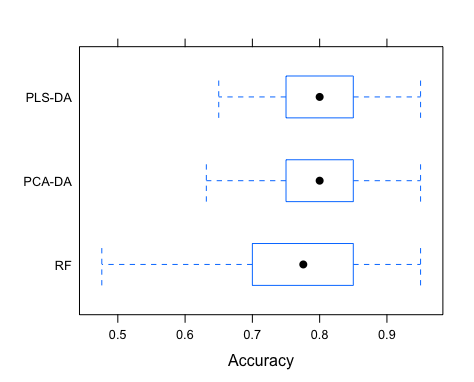
It is clear that the long RF run did not translate into a excelling performance, quite the opposite. Although in average all three models have similar performances, the RF displays a much larger variance in accuracy, which is of course a concern if we seek a robust model. In this case PLS-DA and PCA-DA exhibit the best performance (63-95% accuracy) and either model would do well in diagnosing cancer in new serum samples.
To conclude, we will determine the ten proteins that best diagnose cancer using the variable importance in the projection (ViP), from both the PLS-DA and PCA-DA. With varImp, this is given in relative levels (scaled to the range 0-100).
| plot(varImp(mod1), 10, main = "PLS-DA") | |
| plot(varImp(mod2), 10, main = "PCA-DA") |


Very different figures, right? Idiosyncrasies aside, how many PCs did the PCA-DA use? By calling mod2$preProcess, we learn that “PCA needed 82 components to capture 95 percent of the variance”. This is because the PCA pre-processing functionality in caret uses, by default, as many PCs as it takes to cover 95% of the data variance. So, in one hand we have a PLS-DA with five LVs, on the other hand a PCA-DA with 82 PCs. This not only makes PCA-DA cheaply complicated, but arcane at the interpretation level.
The PLS-DA ViP plot above clearly distinguishes V1184 from all other proteins. This could be an interesting cancer biomarker. Of course, many other tests and models must be conducted in order to provide a reliable diagnostic tool. My aim here is only to introduce PLS and PLS-DA.
And that’s it for today, I hope you enjoyed. Please drop me a comment or message if you have any suggestion for the next post. Cheers!

Thank you for this post. It is an interesting data set and a good opportunity to apply PLS and the caret package.
LikeLike
Very interesting post. I ‘m quite puzzled by the fact that the ten most important biomarkers of cancers are completely different among approaches. Some proteins should be common, at least V1184, no?
LikeLike
Hi Auguet! As I wrote above, “in one hand we have a PLS-DA with five LVs, on the other hand a PCA-DA with 82 PCs” – keep in mind that the PCA-DA fit is unconstrained! Technically speaking, we should also cross-validate the number of PCs in the PCA, but actually I don’t know how to do it with the functions above – wrapping them into a function along with prcomp should do it. I am very positive that the optimal number of PCs for the PCA-DA is lower than that, and the resulting ViP should be likely similar (assuming the performance is also similar!). Cheers
LikeLike
Very interesting post! I wonder what is the difference (if any!) between PLS and Redundancy Analysis (RA). From what I understand, both procedures do something like a PCA, but constraining the PCs such that the variance explained AND the fit to the dependent variable(s) is maximized. Please comment.
LikeLike
Hi Gerardo, thanks! That is a very good question, I actually don’t know what RA is. From what I read over different webpages, it seems that RA relates two datasets X and Y. Note that this Y is no longer a single variable, but multiple! This RA is very much like canonical correlation analysis (CCA) but
– using the same decomposition that underlies PCA and PLS, as you correctly pointed out
– maximizing the correlation of the resulting PCs in X (resp. PCs in Y) with the variables in Y (resp. X)
If so, it only differs from O2PLS in that O2PLS maximizes correlation between PCs (PC1X with PC1Y, PC2X with PC2Y, and so on), similarly to CCA. I hope this helps?
Francisco
LikeLike
i have read your notes on PCA nad PLS.both are very interesting and useful for me.you gave me the rough idea of PLS.if you dont mind can you teach me about the PLS and the process how to compute the PLS manually without using R. i mean on the small data.i need to calculate it to really understand how PLS regresion works.need your help. thank you so much.
LikeLike
The RF example returns an error:
Model cranger is not in caret’s built-in library
LikeLike
Hey Andem, thanks for the comment! I presume it is a problem from the current caret release – it happened to me before and I posted in the Issues tab over the respective GitHub page, topepo/caret/caret . Is your caret version the latest? Can you try downloading the dev version?
LikeLiked by 1 person
current ‘caret’ dev version 6.0-81 throws error on mod3: “Error: The tuning parameter grid should have columns mtry, splitrule, min.node.size”. I’ll roll back with ‘checkpoint’ to this post’s date to fix.
LikeLike
Hi Rich, please let me know if you worked it out. That seems to be a problem from the ranger package, for random forests.
LikeLiked by 1 person
To solve the “Error: The tuning parameter grid should have columns mtry, splitrule, min.node.size” in caret 6.0-84 and R version 3.6.1 (2019-07-05) when building mod3 for RF you have to add the missing columns splitrule and min.node.size, e.g. tuneGrid = data.frame(mtry = seq(10,.5*ncol(arcene), length.out = 6), splitrule = “gini”, min.node.size = 1) .
LikeLiked by 1 person
Thanks a lot for this article which I found really helpful! I have a question: where, in `train()`, did you specify that the “one SE” rule would be applied? I can’t find that in the documentation.
LikeLike
Hey Joe, thanks for the feedback! That should come as an argument to trainControl(), that in turned is passed as trControl inside train(). Here is an example:
ctrl <- trainControl("repeatedcv", …, selectionFunction = "oneSE")
model <- train(x, y, …, trControl = ctrl)
Hope this makes sense! Cheers,
Francisco
LikeLike
Hi Francisco. I’d actually just missed it at the very end of the code box, so thanks for the pointer!
I have a couple of other questions regarding cross-validation if you don’t mind. Firstly, after running your code and model above and then calling “mod1”, I get as part of the output:
“Resampling: Cross-Validated (10 fold, repeated 1 times)”
Why not 5 fold repeated 10 times as I thought you had specified?
Secondly, you point out that with this relatively small sample size it’s sensible to increase the number of repetitions to compensate for having few folds. So, if you had a larger sample size eg n=1000, to what extent would you increase the number of folds?
Many thanks and apologies if I have misunderstood!
LikeLike
Hi Joe. That is odd, the lines
myfolds <- createMultiFolds(arcene$class, k = 5, times = 10)
control <- trainControl("repeatedcv", index = myfolds, selectionFunction = "oneSE")
should result in a 5-fold cross-validation repeated 10 times, indeed. I will look into it later.
Concerning your second point – that is a good question. There are two key points to bear in mind, 1) the fewer folds you use, the more uncertain your CV estimates will be, and 2) the fewer observations per fold, the less representative, and more sensitive it will be to outliers. In the extreme case of the latter, some people advocate in favour of leave-one-out (LOO) CV, with treats each separate observation as a fold. Again, if you have one single outlier, it will drive your average CV metric towards wild values. Then again for small sample sizes, some people prefer bootstrap methods that incorporate repeated sampling. There is plenty of methods to choose from.
If I had n=1000, and furthermore assuming the sample to be rather homogeneous, I would use a 10x CV without repetitions. Each fold would include 100 observations which would in principle be fairly representative of the whole set, and provide a fairly robust mean/SE CV metric from all 10 estimates.
Concluding, there is no optimal method! Try different approaches with caution! Hope this helps,
Francisco
EDIT I have just looked into the 10-fold x1 problem – if you look into `mod1$resample` you should have a total of 50 resample estimates and not 10. Moreover, the column `Resample` clearly shows the fold number goes up to five, and the `Rep` to 10 as expected. That model information is simply not accurate, so ignore it!
LikeLike
Hi Francisco,
What you are saying about the cross-validation is very interesting. I have two questions:
1. can you recommend me literature about cross-validation related to predictive or classification models.
2. I was reading somewhere that cross-validation is really pseudo-randomization. how can we be aware of the effects of this? Is there any metric?
Thanks,
Natalia
LikeLike
I recommend Applied Predictive Modeling by Max Kuhn, there is a good section about resampling incl. cross-validation.
The CV procedure hides some random data from the model, which has to accurately predict the associated response or outcome. It simulates the case of having a model today (so to speak) to predict on data from tomorrow, that still does not exist. The reference above should give you a good idea about CV in general! To be aware of the effects you have to experiment with it. Hope this helps
Best,
Francisco
LikeLike
Thanks Francisco, that’s a perfect explanation. Looks like I found a minor bug in Caret then, but fortunately nothing to worry about!
LikeLike
Hello Francisco,
I’ve been having a discussion with some colleagues about the rule of thumb in PCA which is not to have more predictors than observations. Anybody can run a PCA anyways but can we trust these results? If you know any literature that talks about it and you can suggest it I’ll appreciate it. 🙂
LikeLike
Hi Natalia,
When you have more predictors than observations, your data set is (following the algebra terminology) called singular. In practice, this means you can virtually find any pattern in the data set just because you have so many variables, making it harder to analyse it. When handling such data sets, PCA is actually helpful! PCA helps reducing the complexity of the data by lowering the number of variables down to a few surrogate variables called principal components. Finally, answering your question: you can only trust the results if you know exactly what goes in. Knowing the principles outlined above, e.g. that PCA aims at maximising the spread of the data points, should be enough to understand minimally well what is going on and how to interpret results.
As for literature, check the Nature link above! Best,
Francisco
LikeLike
Hi Francisco,
Thank you for the answer! I’ll pass it around to my group to keep the discussion. So, sorry to bother you again but I haven’t been able to find the Nature link you mentioned in your post..
LikeLike
Hi Natalia!
Sorry, the link is in my PCA post, here you go:
https://www.nature.com/articles/nbt0308-303
Please do not confuse PCA for PLS! Let me know if I can help further.
Francisco
LikeLike
Hello thanks you for all but I get errors with train :
Something is wrong; all the Accuracy metric values are missing:
Accuracy Kappa
Min. : NA Min. : NA
1st Qu.: NA 1st Qu.: NA
Median : NA Median : NA
Mean :NaN Mean :NaN
3rd Qu.: NA 3rd Qu.: NA
Max. : NA Max. : NA
NA’s :20 NA’s :20
LikeLike
Hi Seb, sorry but that is not sufficiently informative. That could be because of various many things, for example if your data contains NAs or if the target variable is misrepresented. Did your model throw any error messages during training?
LikeLike
Good morning, in fact I taken your dataset (arcene) and it does not work. Maybe you used the old version of the caret library ?
LikeLike
For sure it was an older version, but most models and options are still maintained (https://cran.r-project.org/web/packages/caret/vignettes/caret.html).
I just tested the code and got the following warning:
Error: mtry can not be larger than number of variables in data. Ranger will EXIT now.
Did you also get this? Please replace “ranger” with “rf” for now – this is a slightly different random forests package. With this change it all works for me using caret_6.0-86.
LikeLike
Same problem with caret_6.0-88 and I tried to install caret_6.0-86 :
install.packages(“caret_6.0.86.tar.gz”)
Warning in install.packages :
package ‘caret_6.0.86.tar.gz’ is not available (for R version 3.6.3)
😞
LikeLike
Do not worry, nothing we cannot fix. So I just ran the script top to bottom, and it works. However, there are some warnings on mtry values larger than the number of variables – this seems to be a problem of
tuneLength. In any case it should work with the said version. Please use the following to install it from the archive:packageurl <- “https://cran.r-project.org/src/contrib/Archive/caret/caret_6.0-86.tar.gz”
install.packages(packageurl, repos=NULL)
Hope this works. Best, Francisco
LikeLike
Hello, thanks you too much. rStudio does not work but R does !!!!! thanks you and sorry to annoy you. Best regards!
LikeLike