Great strides in artificial intelligence development during the last five years produced agents that are now commonplace at work and home. It is humbling to note that virtually all frontier large language models today trace back to a preprint introducing the transformer neural network architecture¹ – a fifteen-page paper that profoundly rocked the world through waves of excitement and angst.

This paradigm shift in model design has also heavily influenced computer vision, leading to a surge in vision-language models (VLMs). Not only can such systems easily generalize across tasks such as segmentation, depth estimation and image generation or editing², they have also blown legacy models out of the water in object detection benchmarks, with little to no fine-tuning³.

However, it should not be lightly assumed that the transformer architecture is the only path forward to a more meaningful, cost-effective or even better-performing AI – not when we are still having trouble counting “r” in the word strawberry. Neuromorphic computation⁴, photonic neural networks⁵, JEPA⁶ and many other techniques have recently shown us different ways to design and implement intelligent systems that produce optimal solutions for a variety of problems.

Today I want to focus on a topic from a timeless book that inspired me to think differently and, particularly, to effectively apply a first principles approach to problem-solving. The topic is edge detection, and that book is Vision, by David Marr⁷. Just as On the Origin of Species⁸ and On Growth and Form⁹, this is yet another masterpiece that brought together different disciplines – in this case neurophysiology and computer vision – to revolutionise science.

In this blog post we will define and compare algorithms for image edge detection, and explore their remarkable similarity with neurophysiological readings.

Introduction

Modern computer vision is deeply rooted in Marr’s pioneering work. To understand any information-processing system, Marr argued, one must describe it at three interdependent levels of analysis:

• The computational level – what problem is being solved and why (e.g. edge detection)
• The algorithmic level – how it is solved, and what representations and procedures are used (e.g. the Laplacian transform)
• The implementational level – where it is physically realised (e.g. in vivo, in silico)

This layered thinking is what makes the book so enduring. Marr was not merely describing the visual system, he was arguing that to truly understand it you had to explain it at all three levels simultaneously. The book also features memorable passages on random dot stereograms¹⁰, binocular disparity and motion perception – overall, highly recommended for science enthusiasts.

Let us now introduce the key concepts underlying edge detection that leveraged this structured approach, to gain a better understanding of how it can be solved in practice.

Zero-crossing ✏️

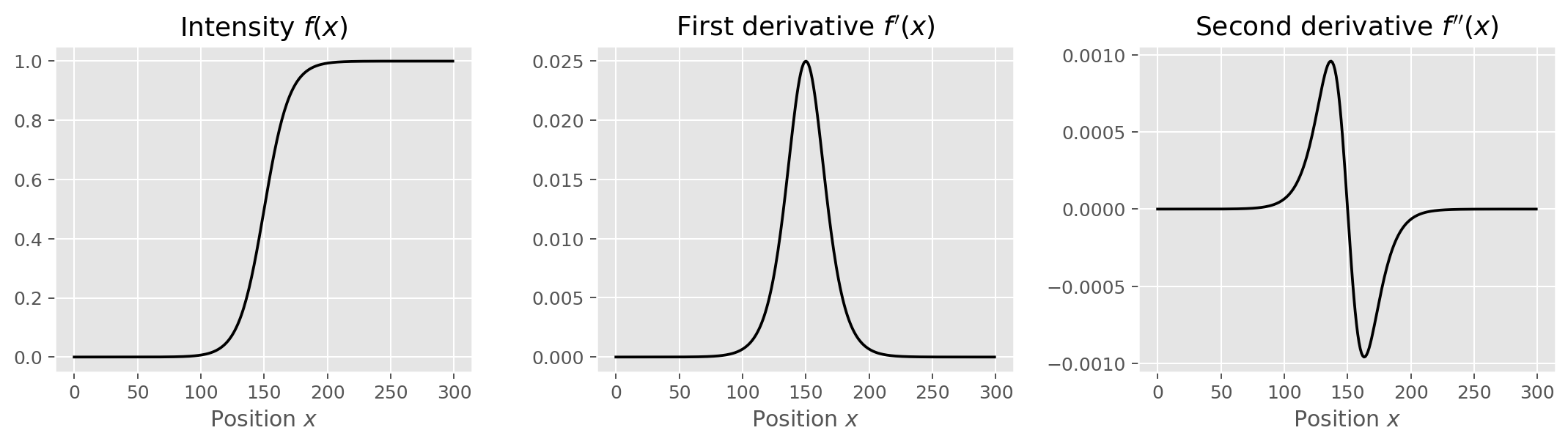
From a computational perspective, edges are fundamentally spatial discontinuities in images. If for a brief moment we consider a simple greyscale image, edges are wherever dark-to-light and light-to-dark transitions occur, in whatever direction.

Because such transitions mathematically translate to local changes in pixel intensity, the most natural approach to identify edges is to compute image gradients, the two-dimensional equivalent of the derivative. The first derivative of image intensity evaluated across an edge produces a peak (for a dark-to-bright transition) or a trough (for a bright-to-dark transition), depending on the direction. However, the second derivative provides not only the means to identify both transition types, but also a beautifully simple detection mechanism: it crosses zero at the precise location of the edge. This is the essence of the zero-crossing.

Marr and Hildreth formalised this insight by proposing the Laplacian of Gaussian (LoG) as the operator of choice¹¹. The Laplacian is the sum of second partial derivatives in both spatial dimensions:

Applied directly to a noisy image, the Laplacian amplifies every small intensity fluctuation. The Gaussian pre-filter solves this by smoothing the image at a chosen scale before differentiation. Because convolution is associative, the two steps can be combined into a single kernel – the LoG, also denoted :

This kernel, which resembles an inverted sombrero and is sometimes called the Mexican hat wavelet, produces a response that crosses zero exactly at an intensity edge. The width of the Gaussian determines the scale of detection: small preserves fine detail, large captures only coarse structure. Marr argued that the visual system operates simultaneously at multiple scales – an idea that would later resonate in scale-space theory and, much later, in the multi-scale feature maps of deep convolutional networks.

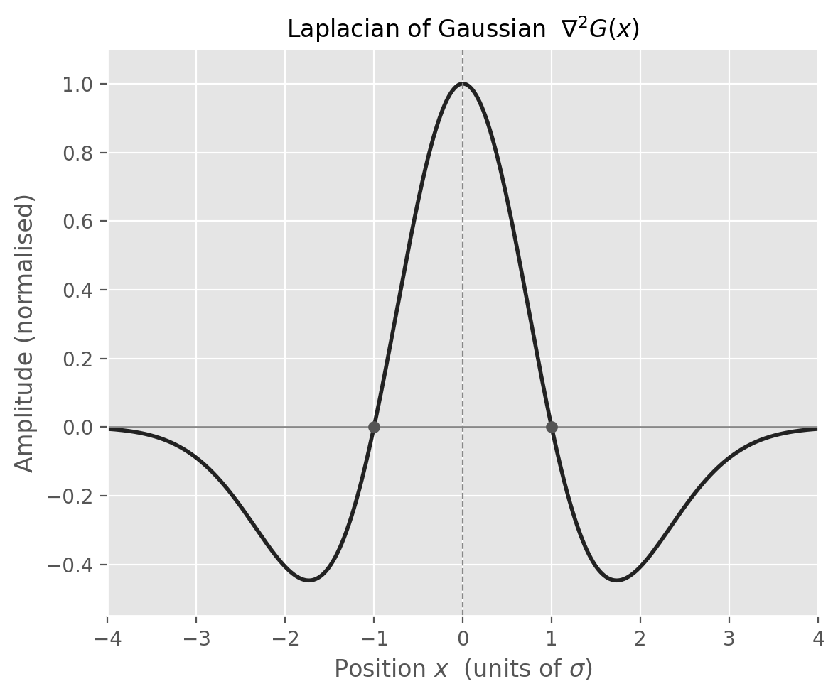
Marr went further and showed that the centre-surround organisation of retinal ganglion cell receptive fields – which he modelled as a Difference of Gaussians (DoG), the difference between a narrow excitatory Gaussian and a broader inhibitory one – is a close biological approximation of the LoG. Put differently, your retina is already computing zero-crossings before the signal ever reaches the visual cortex. The agreement between computational predictions and in vivo electrophysiological measurements, documented in Vision (p. 64), remains one of the most compelling examples of theory meeting experiment in all of neuroscience.

Zero-crossings are theoretically elegant, but the workhorse operators most computer-vision tools reach for – including, as we will see, the Canny detector itself – operate on first-derivative gradients. Let us look at those.

Image gradients 📐

In practice, image gradients are computed using convolution filters – small kernels that slide across the image and produce a weighted local sum at each pixel, as illustrated in my post on convolutional neural networks. The two most widely used first-order gradient operators are:

Sobel: weights the central row and column more heavily, providing a modest degree of smoothing:

Prewitt: weights all neighbours equally:

In both cases the gradient magnitude at each pixel is , and the gradient direction is . Where the magnitude is large, a transition is occurring; where it is small, the neighbourhood is uniform.

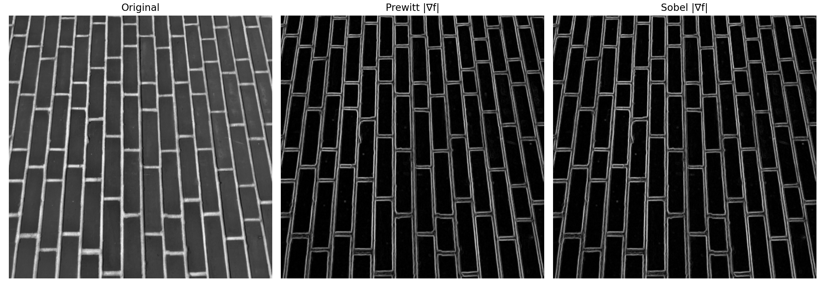
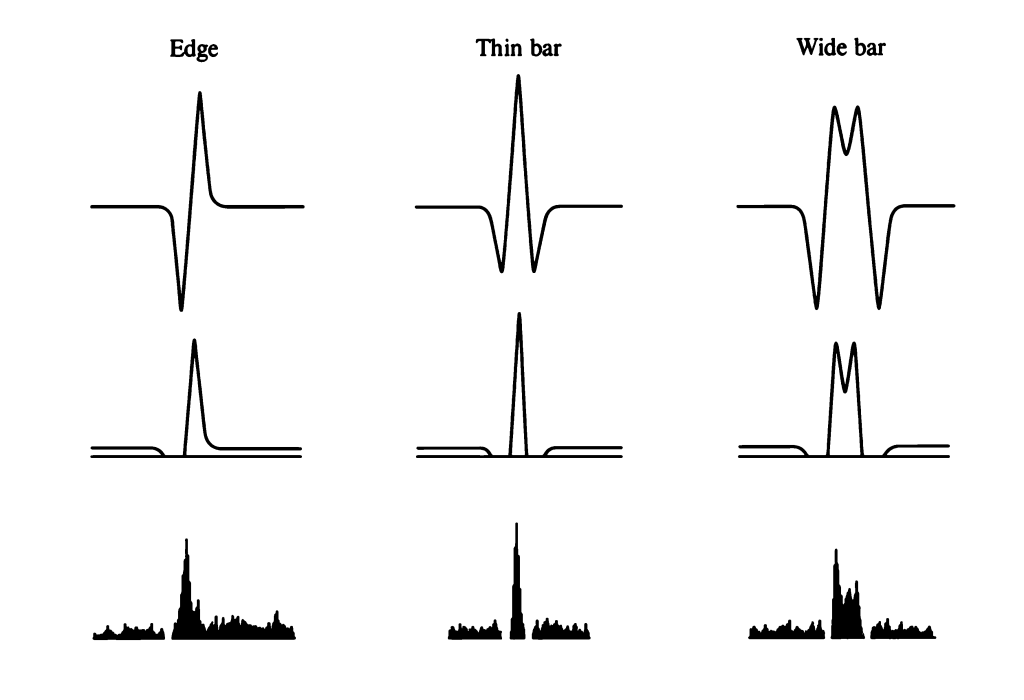
The limitation of these operators is that they are sensitive to noise and produce thick, diffuse edges. Every pixel with a large gradient is flagged regardless of whether it truly lies on the edge or merely near it. This is precisely the problem that John Canny set out to solve.

Canny edge detection 🔍

Published in 1986, John Canny’s paper A Computational Approach to Edge Detection¹² remains one of the most cited works in computer vision. Canny framed edge detection as an explicit optimisation problem and derived a detector that simultaneously maximises three criteria: i) good detection (few missed edges, few “false alarms”), ii) good localisation (detected edges close to true edges), and iii) single response (one response per edge, not many). The resulting algorithm is a four-step pipeline outlined below:

Step 1 – Gaussian smoothing

As with the LoG, the first step is to suppress noise by convolving the image with a Gaussian kernel of width . The choice of directly governs the trade-off between noise suppression and fine detail preservation. A larger removes more noise but blurs genuine edges.

Step 2 – Gradient computation

The smoothed image is then differentiated, typically using Sobel kernels – to obtain the gradient magnitude and direction at every pixel.

Step 3 – Non-maximum suppression (NMS)

This step thins the edges. For each pixel, Canny checks whether its gradient magnitude is a local maximum along the gradient direction – that is, whether it is larger than its two neighbours in the direction . If it is not, it is suppressed to zero. The result is a set of thin, one-pixel-wide candidate edges.

Step 4 – Hysteresis thresholding

The final step uses two thresholds, and , to prune candidate pixels. A pixel whose gradient magnitude exceeds is accepted as an edge, and conversely a pixel below is rejected. A pixel between the two thresholds is accepted only if it is connected, directly or through other such pixels, to a strong edge pixel. This connectivity analysis – the defining feature of hysteresis – ensures that long, continuous edges are preserved even when their local gradient fluctuates, while isolated noise responses are discarded. For a more visual understanding of NMS and hysteresis I recommend reading the Canny edge detection documentation from OpenCV.

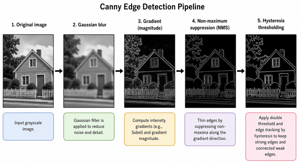
The elegance of Canny lies in how each step addresses a specific failure mode of earlier operators. In essence Gaussian smoothing tackles noise, NMS tackles thick edges and hysteresis tackles the false edge / broken edge trade-off that a single threshold cannot solve.

Let’s get started with Python

Time to practice! We will first build the separate components (Gaussian blur, Sobel gradients, LoG zero-crossings), then run the full Canny pipeline and explore how its parameters trade off recall against noise. We will use opencv and scikit-image alongside the usual suspects numpy and matplotlib. You can install all packages using the following shell command:

pip install opencv-python scikit-image matplotlib numpy

Image loading and preprocessing

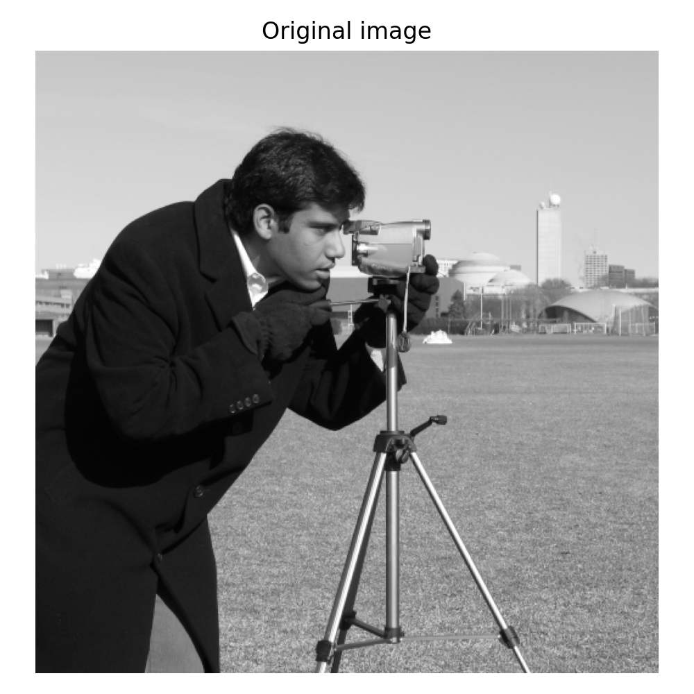
We start by loading a greyscale image. For demonstration purposes I use a stock picture from scikit-image – feel free to use any other image of your choice.

import cv2
import numpy as np
import matplotlib.pyplot as plt
from skimage import data
from scipy.ndimage import gaussian_laplace
# Load a greyscale test image (uint8, values 0–255)
image = data.camera()
 
fig, ax = plt.subplots(figsize=(5, 5))
ax.imshow(image, cmap='gray')
ax.set_title('Original image')
ax.axis('off')
plt.tight_layout()
plt.show()

The Laplacian of Gaussian and zero-crossings

Let us inspect the LoG response and its zero-crossings – the theoretical backbone we discussed earlier.

# LoG: positive sigma = apply Gaussian of that std, then Laplacian
log_response = gaussian_laplace(image.astype(float), sigma=2.0)
 
# Zero-crossings: sign changes between neighbouring pixels
def zero_crossings(log_img):
    """Return a binary mask of zero-crossing locations."""
    zc = np.zeros_like(log_img, dtype=bool)
    # Check horizontal and vertical sign changes
    for shift in [(0, 1), (1, 0)]:
        shifted = np.roll(log_img, shift=shift, axis=(0, 1))
        zc |= (np.sign(log_img) != np.sign(shifted))
    return zc
 
zc_mask = zero_crossings(log_response)
 
fig, axes = plt.subplots(1, 2, figsize=(10, 4))
axes[0].imshow(log_response, cmap='RdBu_r')
axes[0].set_title('LoG response (σ=2.0)')
axes[0].axis('off')
axes[1].imshow(zc_mask, cmap='gray')
axes[1].set_title('Zero-crossings')
axes[1].axis('off')
plt.tight_layout()
plt.show()

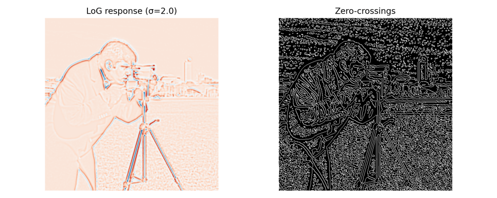
Notice how the zero-crossing map already captures much of the scene’s edge structure, but it is sensitive to low-level noise and retains spurious responses in flat regions. This motivates the additional refinement steps of the Canny algorithm.

Gaussian smoothing and gradient computation

Before running the full Canny pipeline, it is instructive to inspect the intermediate steps. Here we apply a Gaussian blur and then compute Sobel gradients manually.

# Gaussian blur — sigma controlled by ksize (must be odd) and sigmaX
blurred = cv2.GaussianBlur(image, ksize=(5, 5), sigmaX=1.4)
 
# Sobel gradients in x and y
Gx = cv2.Sobel(blurred, cv2.CV_64F, dx=1, dy=0, ksize=3)
Gy = cv2.Sobel(blurred, cv2.CV_64F, dx=0, dy=1, ksize=3)
 
# Gradient magnitude
magnitude = np.sqrt(Gx**2 + Gy**2)
magnitude = (magnitude / magnitude.max() * 255).astype(np.uint8)
 
fig, axes = plt.subplots(1, 2, figsize=(10, 4))
for ax, img, title in zip(axes, [blurred, magnitude], ['Gaussian blur (σ=1.4)', '|∇f| - Sobel magnitude']):
    ax.imshow(img, cmap='gray')
    ax.set_title(title)
    ax.axis('off')
plt.tight_layout()
plt.show()

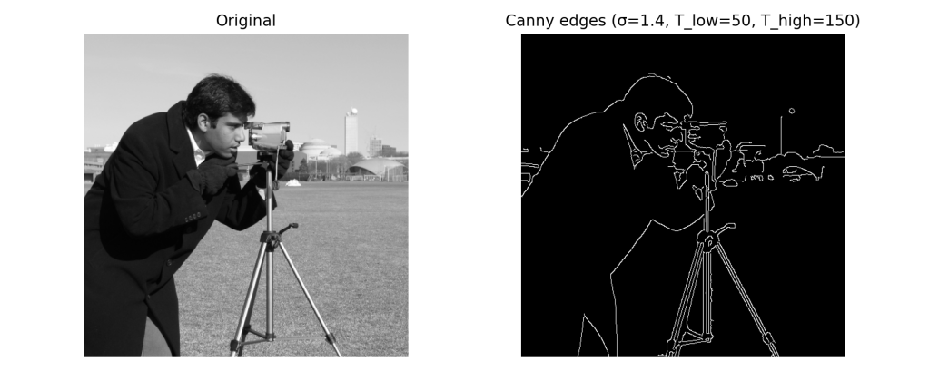
Canny edge detection with OpenCV

The OpenCV Canny() function accepts the image, the two hysteresis thresholds, and an optional aperture size for the Sobel operator. Crucially, the Gaussian smoothing step should be applied manually beforehand so you have full control over .

def run_canny(image, sigma, t_low, t_high, aperture=3):
    """Apply Gaussian blur then Canny edge detection."""
    # Kernel size: 2 * ceil(3*sigma) + 1 ensures the kernel covers ±3σ
    ksize = 2 * int(np.ceil(3 * sigma)) + 1
    blurred = cv2.GaussianBlur(image, (ksize, ksize), sigmaX=sigma)
    edges = cv2.Canny(blurred, threshold1=t_low, threshold2=t_high, apertureSize=aperture)
    return edges
edges = run_canny(image, sigma=1.4, t_low=50, t_high=150)
fig, axes = plt.subplots(1, 2, figsize=(10, 4))
axes[0].imshow(image, cmap='gray')
axes[0].set_title('Original')
axes[0].axis('off')
axes[1].imshow(edges, cmap='gray')
axes[1].set_title('Canny edges (σ=1.4, T_low=50, T_high=150)')
axes[1].axis('off')
plt.tight_layout()
plt.show()

The effect of hysteresis thresholds

The ratio is at least as important as the absolute values. A common rule of thumb is to use a 2:1 or 3:1 ratio. Let us explore this now.

fig, axes = plt.subplots(2, 3, figsize=(14, 8))
configs = [
    (1.4, 20, 60, '↑ Recall, ↑ Noise\nσ=1.4, T=20/60'),
    (1.4, 50, 150, 'Balanced\nσ=1.4, T=50/150'),
    (1.4, 100, 200, '↓ Recall, ↓ Noise\nσ=1.4, T=100/200'),
    (0.5, 50, 150, 'Fine scale\nσ=0.5, T=50/150'),
    (2.0, 50, 150, 'Coarse scale\nσ=2.0, T=50/150'),
    (4.0, 50, 150, 'Very coarse scale\nσ=4.0, T=50/150'),
]
 
for ax, (sigma, tl, th, title) in zip(axes.ravel(), configs):
    result = run_canny(image, sigma=sigma, t_low=tl, t_high=th)
    ax.imshow(result, cmap='gray')
    ax.set_title(title, fontsize=9)
    ax.axis('off')
 
plt.tight_layout()
plt.show()

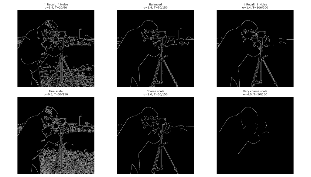
The top row demonstrates the threshold effect – lower thresholds recover more edges but also more noise, higher thresholds yield cleaner output at the cost of broken contours. The bottom row shows the scale effect governed by – at small scales the detector responds to fine texture and noise, at large scales only the dominant structural boundaries survive.

Overlaying edges on the original image

A useful visualisation is overlaying detected edges on the original image. This facilitates the quality assessment of our workflow.

# Convert to RGB so we can draw edges in red
overlay = cv2.cvtColor(image, cv2.COLOR_GRAY2RGB)
overlay[edges > 0] = [220, 40, 40] # red edges
 
fig, ax = plt.subplots(figsize=(6, 6))
ax.imshow(overlay)
ax.set_title('Canny edges overlaid (σ=1.4, T=50/150)')
ax.axis('off')
plt.tight_layout()
plt.show()

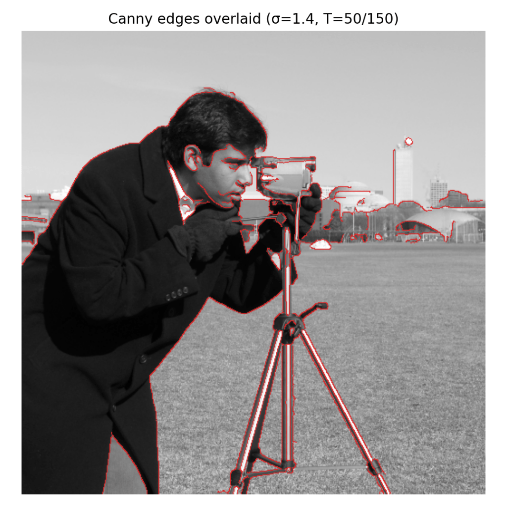
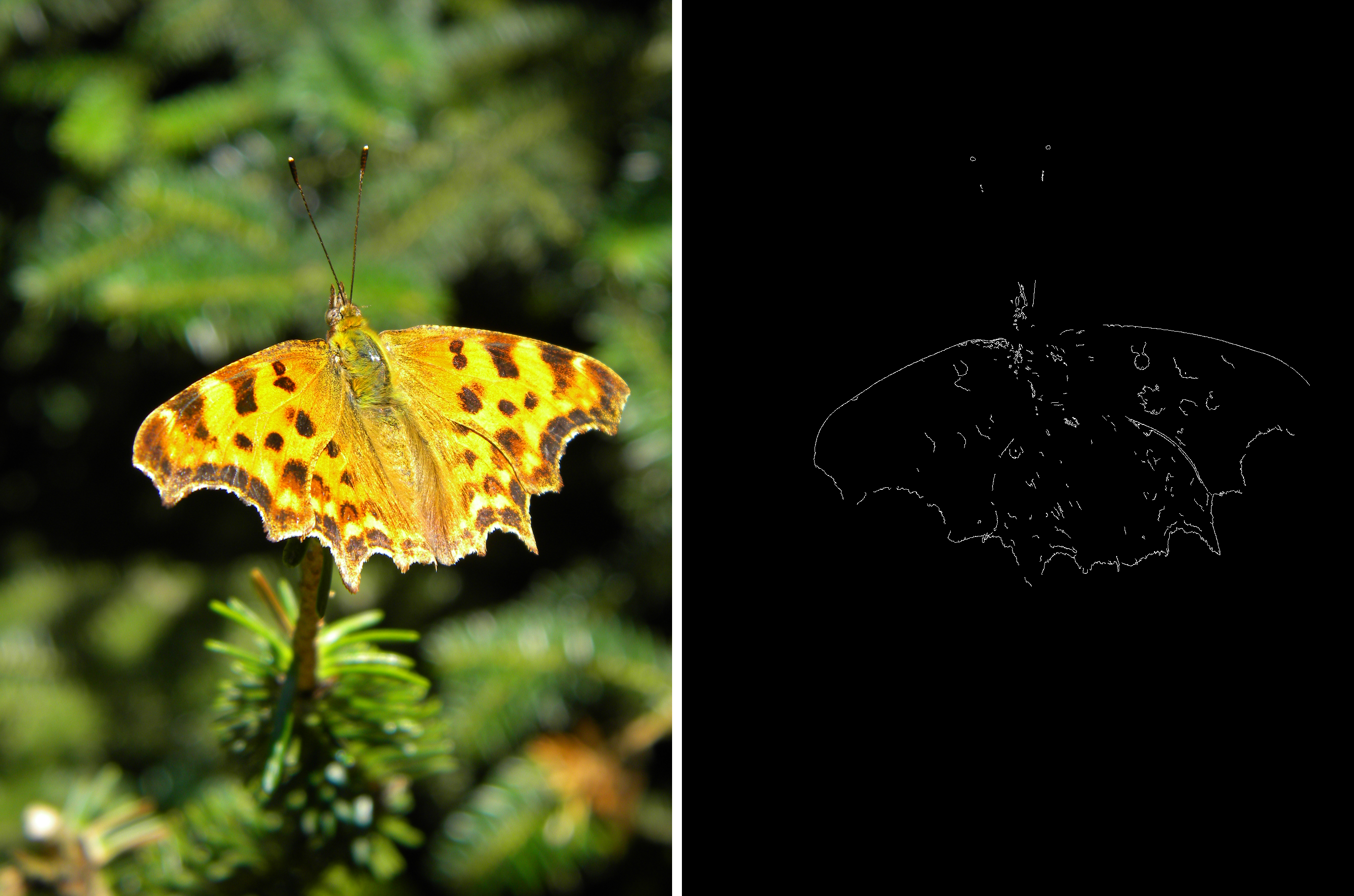
Similarly to the butterfly picture, here we find a solution that precisely identifies the sharpest edges from the image.

Conclusion 🏁

We have traced a line from the centre-surround receptive fields of retinal ganglion cells to the LoG operator and Marr’s zero-crossings, and from there to the Canny detector – one of the most popular algorithms in image processing. The key ideas are worth summarising:

• Edges are zero-crossings of the second derivative of image intensity, a principle Marr derived from first principles and validated against neurophysiology 🧠
• The LoG operator implements this computationally: a Gaussian pre-filter controls scale and suppresses noise, whereas the Laplacian finds sign changes 💻
• Canny refines the idea with NMS for thin, well-localised edges, and hysteresis thresholding to preserve continuous contours without fragmenting them 🏙️

Edge detection may seem like a solved problem in an era of end-to-end learned vision systems, but it remains the conceptual foundation of a surprisingly wide range of techniques. Some practical applications worth exploring on your own include:

• Hough transform for line and circle detection – it operates directly on edge maps
• Contour-based object detection – a classical pre-deep-learning approach that is still competitive in constrained domains
• Medical image segmentation – where edge-based pre-processing still complements learned models for thin-structure detection

That brings us to a close – thanks for reading, I hope this post was insightful and entertaining. Stay curious! 💡

References 📖

1. Vaswani, A., Shazeer, N., Parmar, N., Uszkoreit, J., Jones, L., Gomez, A. N., Kaiser, Ł., & Polosukhin, I. (2017). Attention Is All You Need. arXiv:1706.03762. ↩︎
2. Vision Banana team, Google DeepMind (2026). Image Generators are Generalist Vision Learners. arXiv:2604.20329. ↩︎
3. Robicheaux, P. et al. (2025). RF-DETR: Neural Architecture Search for Real-Time Detection Transformers. arXiv:2511.09554 (ICLR 2026). ↩︎
4. Kudithipudi, D. et al. (2025). Neuromorphic computing at scale. Nature 637, 801–812. ↩︎
5. Ashtiani, F., Idjadi, M. H., & Kim, K. (2026). Integrated photonic neural network with on-chip backpropagation training. Nature 651, 927–932. ↩︎
6. Assran, M. et al. (2023). Self-Supervised Learning from Images with a Joint-Embedding Predictive Architecture (I-JEPA). arXiv:2301.08243. ↩︎
7. Marr, D. (1982). Vision: A Computational Investigation into the Human Representation and Processing of Visual Information. W. H. Freeman; reissued by MIT Press (2010). ↩︎
8. Darwin, C. (1859). On the Origin of Species by Means of Natural Selection. John Murray, London. ↩︎
9. Thompson, D’A. W. (1917). On Growth and Form. Cambridge University Press. ↩︎
10. Julesz, B. (1971). Foundations of Cyclopean Perception. University of Chicago Press. ↩︎
11. Marr, D., & Hildreth, E. (1980). Theory of edge detection. Proceedings of the Royal Society of London B, 207(1167), 187–217. ↩︎
12. Canny, J. (1986). A Computational Approach to Edge Detection. IEEE Transactions on Pattern Analysis and Machine Intelligence, PAMI-8(6), 679–698. ↩︎

• Python